t <-t.test(mg2$Mg2, mg2$control)library(report)report(t)
Effect sizes were labelled following Cohen's (1988) recommendations.
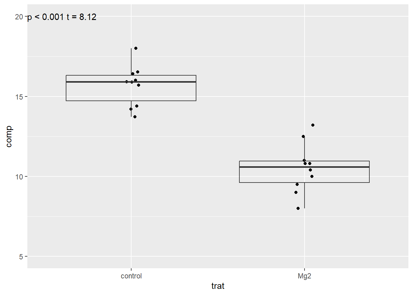
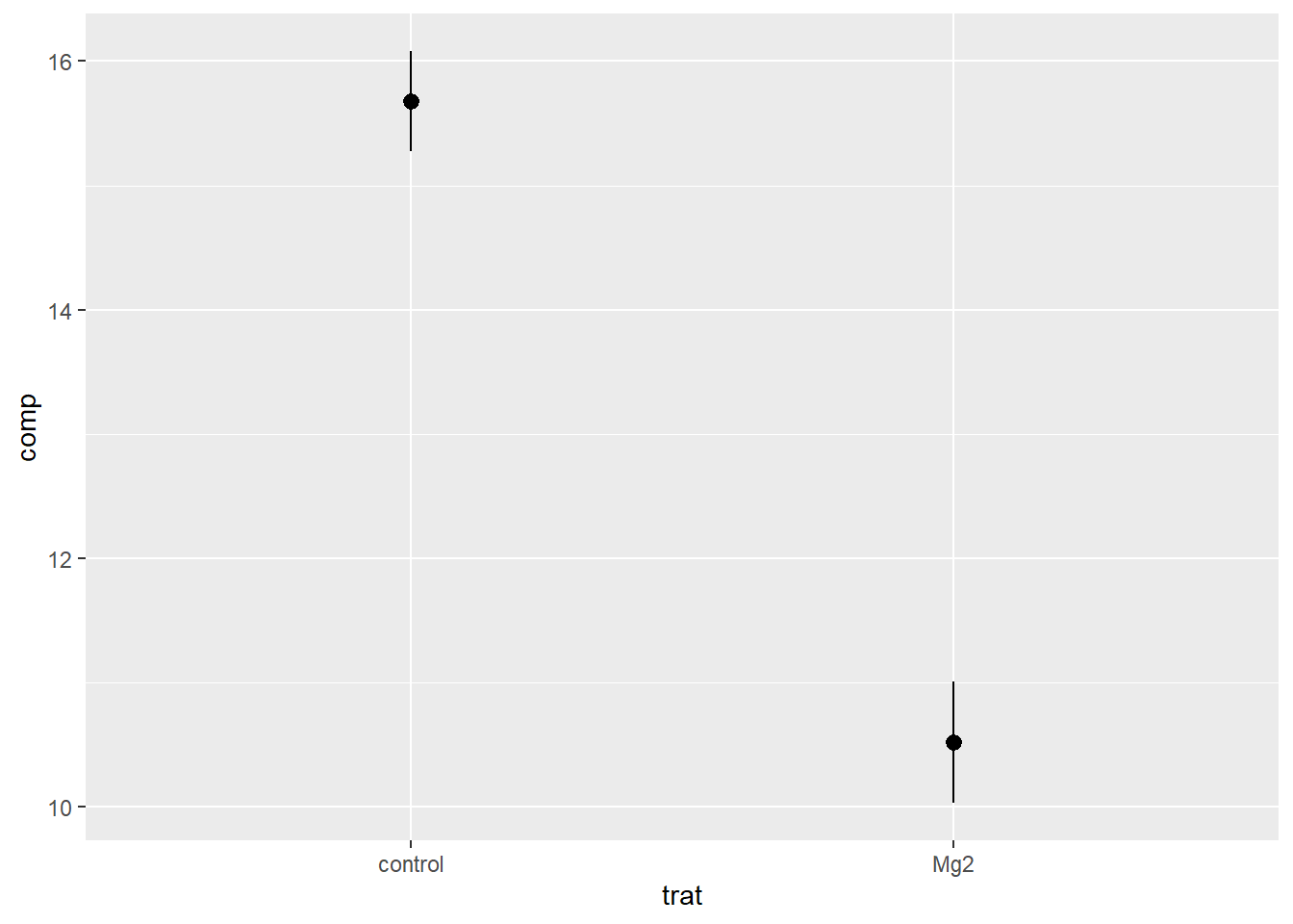
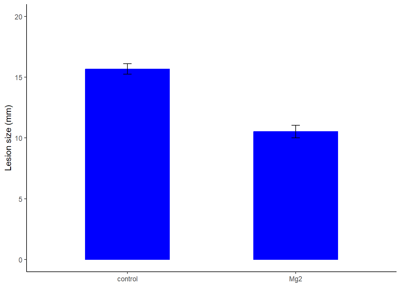
The Welch Two Sample t-test testing the difference between mg2$Mg2 and
mg2$control (mean of x = 10.52, mean of y = 15.68) suggests that the effect is
negative, statistically significant, and large (difference = -5.16, 95% CI
[-6.49, -3.83], t(17.35) = -8.15, p < .001; Cohen's d = -3.65, 95% CI [-5.12,
-2.14])
t <-t.test(mg2$Mg2, mg2$control, paired = F)library(report)report(t)
Effect sizes were labelled following Cohen's (1988) recommendations.

The Welch Two Sample t-test testing the difference between mg2$Mg2 and
mg2$control (mean of x = 10.52, mean of y = 15.68) suggests that the effect is
negative, statistically significant, and large (difference = -5.16, 95% CI
[-6.49, -3.83], t(17.35) = -8.15, p < .001; Cohen's d = -3.65, 95% CI [-5.12,
-2.14])
Homocedesticidade attach separa as variaveis
attach(mg2) # vamos facilitar o uso dos dadosvar.test(Mg2, control)
    F test to compare two variances

data:  Mg2 and control
F = 1.4781, num df = 9, denom df = 9, p-value = 0.5698
alternative hypothesis: true ratio of variances is not equal to 1
95 percent confidence interval:
 0.3671417 5.9508644
sample estimates:
ratio of variances
          1.478111
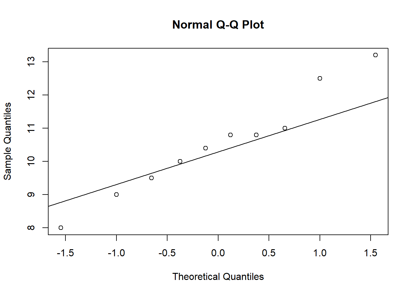
Testar normalidade
shapiro.test(Mg2)
    Shapiro-Wilk normality test

data:  Mg2
W = 0.97269, p-value = 0.9146
shapiro.test(control)
    Shapiro-Wilk normality test

data:  control
W = 0.93886, p-value = 0.5404
    F test to compare two variances

data:  Aided1 and Unaided
F = 0.17041, num df = 9, denom df = 9, p-value = 0.01461
alternative hypothesis: true ratio of variances is not equal to 1
95 percent confidence interval:
 0.04232677 0.68605885
sample estimates:
ratio of variances
         0.1704073
shapiro.test(Aided1)
    Shapiro-Wilk normality test

data:  Aided1
W = 0.92775, p-value = 0.4261
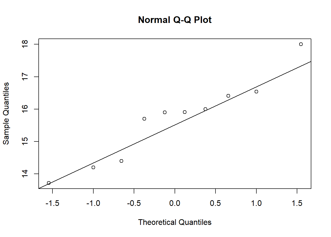
shapiro.test(Unaided)
    Shapiro-Wilk normality test

data:  Unaided
W = 0.87462, p-value = 0.1131
report(t_escala)
Effect sizes were labelled following Cohen's (1988) recommendations.
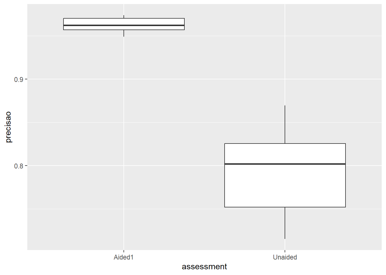
The Paired t-test testing the difference between Aided1 and Unaided (mean
difference = 0.18) suggests that the effect is positive, statistically
significant, and large (difference = 0.18, 95% CI [0.11, 0.26], t(9) = 5.94, p
< .001; Cohen's d = 1.88, 95% CI [0.81, 2.91])
wilcox.test(Aided1, Unaided)
    Wilcoxon rank sum exact test

data:  Aided1 and Unaided
W = 100, p-value = 1.083e-05
alternative hypothesis: true location shift is not equal to 0