Quando os fatores do tratamento é quantitativo nós fazemos análise de regressão.
coeficiente angular: da linha do gráfico da regressão.
a pergunta: a uma tendencia em declinar ou aumentar?
queremos saber se a linha é diferente do angulo zero, que seria reta.
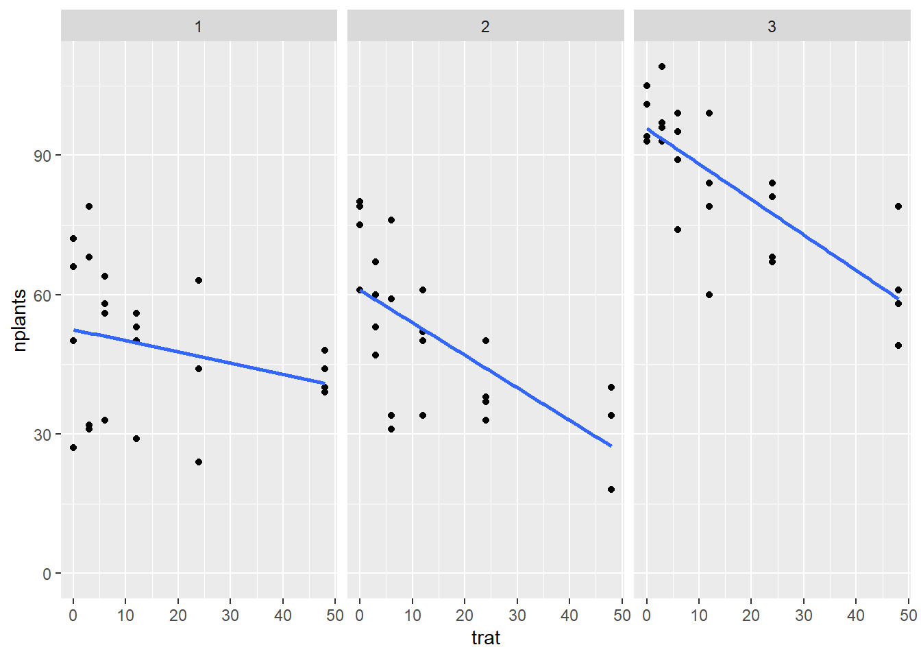
Geom_smooth coloca a linha.
library(readxl)library(tidyverse)library(ggplot2)estande <-read_excel("dados-diversos.xlsx", "estande")estande |>ggplot(aes(trat, nplants))+geom_point()+facet_wrap(~exp)+ylim(0,max(estande$nplants))+geom_smooth(se = F, method="lm")#para a colocar a linha e lm para deixar em padrão linear.
3
exp1 <- estande |>filter(exp ==1) m1 <-lm(nplants ~ trat, data = exp1)#nplants é a resposta em função do tratsummary(m1)
Call:
lm(formula = nplants ~ trat, data = exp1)
Residuals:
Min 1Q Median 3Q Max
-25.500 -6.532 1.758 8.573 27.226
Coefficients:
Estimate Std. Error t value Pr(>|t|)
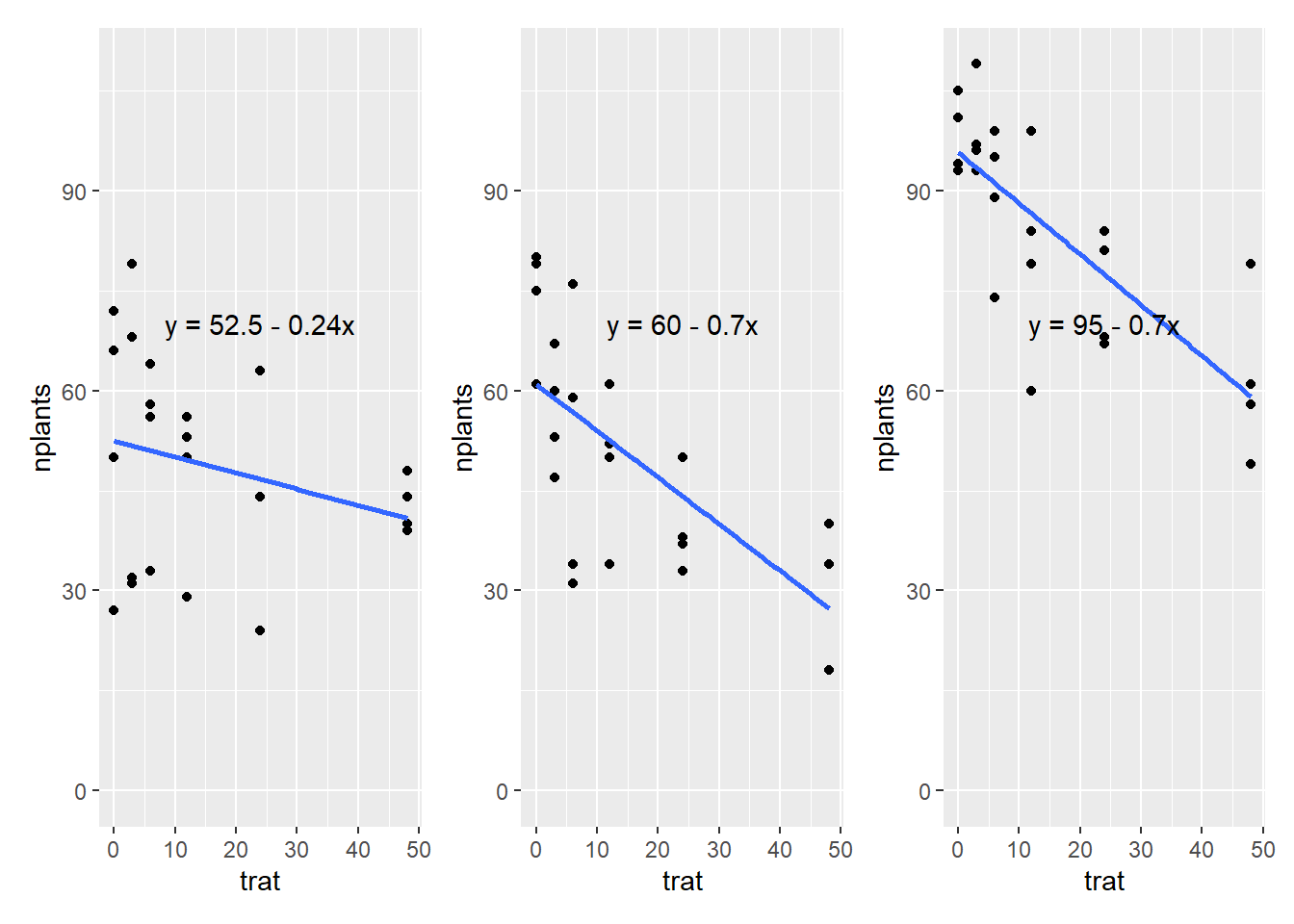
(Intercept) 52.5000 4.2044 12.487 1.84e-11 ***
trat -0.2419 0.1859 -1.301 0.207
---
Signif. codes: 0 '***' 0.001 '**' 0.01 '*' 0.05 '.' 0.1 ' ' 1
Residual standard error: 15 on 22 degrees of freedom
Multiple R-squared: 0.07148, Adjusted R-squared: 0.02928
F-statistic: 1.694 on 1 and 22 DF, p-value: 0.2066
exp2 <- estande |>filter(exp ==2) m2 <-lm(nplants ~ trat, data = exp2)#nplants é a resposta em função do tratsummary(m2)
Call:
lm(formula = nplants ~ trat, data = exp2)

Residuals:
     Min       1Q   Median       3Q      Max
-25.7816  -7.7150   0.5653   8.1929  19.2184

Coefficients:
            Estimate Std. Error t value Pr(>|t|)
(Intercept)  60.9857     3.6304  16.798 4.93e-14 ***
trat         -0.7007     0.1605  -4.365 0.000247 ***
---
Signif. codes:  0 '***' 0.001 '**' 0.01 '*' 0.05 '.' 0.1 ' ' 1

Residual standard error: 12.95 on 22 degrees of freedom
Multiple R-squared:  0.4641,    Adjusted R-squared:  0.4398
F-statistic: 19.05 on 1 and 22 DF,  p-value: 0.0002473
exp3 <- estande |>filter(exp ==3) m3 <-lm(nplants ~ trat, data = exp3)#nplants é a resposta em função do tratsummary(m3)
Call:
lm(formula = nplants ~ trat, data = exp3)

Residuals:
     Min       1Q   Median       3Q      Max
-26.5887  -3.9597   0.7177   5.5806  19.8952

Coefficients:
            Estimate Std. Error t value Pr(>|t|)
(Intercept)  95.7500     2.9529  32.425  < 2e-16 ***
trat         -0.7634     0.1306  -5.847 6.97e-06 ***
---
Signif. codes:  0 '***' 0.001 '**' 0.01 '*' 0.05 '.' 0.1 ' ' 1

Residual standard error: 10.53 on 22 degrees of freedom
Multiple R-squared:  0.6085,    Adjusted R-squared:  0.5907
F-statistic: 34.19 on 1 and 22 DF,  p-value: 6.968e-06
library(report)report(m3)
We fitted a linear model (estimated using OLS) to predict nplants with trat
(formula: nplants ~ trat). The model explains a statistically significant and
substantial proportion of variance (R2 = 0.61, F(1, 22) = 34.19, p < .001, adj.
R2 = 0.59). The model's intercept, corresponding to trat = 0, is at 95.75 (95%
CI [89.63, 101.87], t(22) = 32.43, p < .001). Within this model:

  - The effect of trat is statistically significant and negative (beta = -0.76,
95% CI [-1.03, -0.49], t(22) = -5.85, p < .001; Std. beta = -0.78, 95% CI
[-1.06, -0.50])

Standardized parameters were obtained by fitting the model on a standardized
version of the dataset. 95% Confidence Intervals (CIs) and p-values were
computed using a Wald t-distribution approximation.
Os dois métodos são certos, você pode usar uma abordagem ou outra.
No segundo método o experimento é considerado um fator aleatório. e considera o valor dos 3 experimentos juntos. Porém é mais recomendado quando tem mais repetições, 3 é pouco.
library(lme4)#modelo misto porque tem fator fixo e aleatório, no outro regressão só tem fixo, o experimento é o componente aleatório. Vai juntar os 3 experimentos em um modelo só.mix <-lmer(nplants ~ trat + (trat |exp), data = estande)summary(mix)
Linear mixed model fit by REML ['lmerMod']
Formula: nplants ~ trat + (trat | exp)
   Data: estande

REML criterion at convergence: 580.8

Scaled residuals:
    Min      1Q  Median      3Q     Max
-2.0988 -0.6091  0.1722  0.6360  1.9963

Random effects:
 Groups   Name        Variance  Std.Dev. Corr
 exp      (Intercept) 510.68405 22.5983
          trat          0.05516  0.2349  -0.82
 Residual             167.91303 12.9581
Number of obs: 72, groups:  exp, 3

Fixed effects:
            Estimate Std. Error t value
(Intercept)  69.7452    13.2146   5.278
trat         -0.5687     0.1643  -3.462

Correlation of Fixed Effects:
     (Intr)
trat -0.731
optimizer (nloptwrap) convergence code: 0 (OK)
Model failed to converge with max|grad| = 0.00274249 (tol = 0.002, component 1)
library(car)Anova(mix)#aqui da o P-valor, calcula a média do slop dos 3.
modelo linear é um caso especial de glm, que é a familia gaussian.
nplantas= numerica discreta, usa familia poisson
numerica continua = familia gaussian
Fizemos o ajusto modelo aos dados.
glm1 <-glm(nplants ~ trat, family ="gaussian",data=exp3)summary(glm1)
Call:
glm(formula = nplants ~ trat, family = "gaussian", data = exp3)

Deviance Residuals:
     Min        1Q    Median        3Q       Max
-26.5887   -3.9597    0.7177    5.5806   19.8952

Coefficients:
            Estimate Std. Error t value Pr(>|t|)
(Intercept)  95.7500     2.9529  32.425  < 2e-16 ***
trat         -0.7634     0.1306  -5.847 6.97e-06 ***
---
Signif. codes:  0 '***' 0.001 '**' 0.01 '*' 0.05 '.' 0.1 ' ' 1

(Dispersion parameter for gaussian family taken to be 110.9787)

    Null deviance: 6235.8  on 23  degrees of freedom
Residual deviance: 2441.5  on 22  degrees of freedom
AIC: 185.04

Number of Fisher Scoring iterations: 2
glm2 <-glm(nplants ~ trat, family =poisson(link ="log"),data=exp3)AIC(glm1) # quanto menor o aic melhor o modelo
[1] 185.0449
AIC(glm2) # esse modelo deu melhor porque deu menor.
[1] 183.9324
summary(glm2)
Call:
glm(formula = nplants ~ trat, family = poisson(link = "log"),
    data = exp3)

Deviance Residuals:
     Min        1Q    Median        3Q       Max
-2.94600  -0.46988   0.02453   0.61868   2.34657

Coefficients:
             Estimate Std. Error z value Pr(>|z|)
(Intercept)  4.571590   0.029539 154.762  < 2e-16 ***
trat        -0.009965   0.001488  -6.697 2.13e-11 ***
---
Signif. codes:  0 '***' 0.001 '**' 0.01 '*' 0.05 '.' 0.1 ' ' 1

(Dispersion parameter for poisson family taken to be 1)

    Null deviance: 77.906  on 23  degrees of freedom
Residual deviance: 29.952  on 22  degrees of freedom
AIC: 183.93

Number of Fisher Scoring iterations: 4