library(readxl)
library(tidyverse)
library(ggplot2)

estande <- read_excel("dados-diversos.xlsx", "estande")

estande |>
  ggplot(aes(trat, nplants))+
  geom_point()+
  facet_wrap(~exp)+
  ylim(0,max(estande$nplants))+
  geom_smooth(se = F)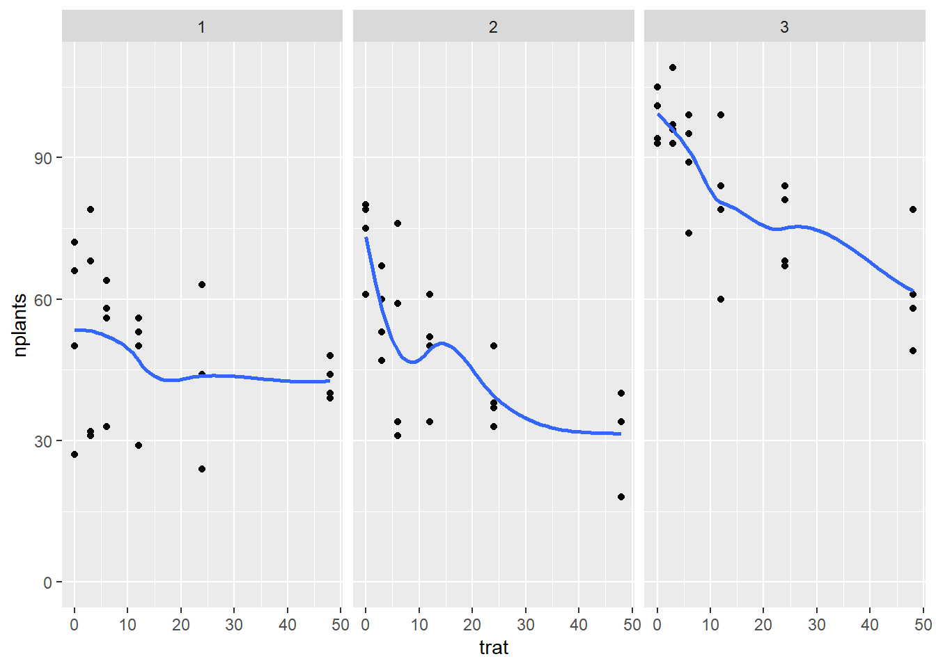
Linha quadrática ou sigmodial a linha não é reta., tem uma curvatura. pq tem mais um fator
y=b1-b2x-cx²
ver se é quadratica ou não antes
verificar os coeficientes
e depois colocar no gráfico a formula
library(readxl)
library(tidyverse)
library(ggplot2)
estande <- read_excel("dados-diversos.xlsx", "estande")
estande |>
ggplot(aes(trat, nplants))+
geom_point()+
facet_wrap(~exp)+
ylim(0,max(estande$nplants))+
geom_smooth(se = F)
estande2 <- estande |>
  filter(exp==2)|>
  group_by(trat) |> #vai eliminar o bloco
  summarise(mean_nplants = mean(nplants))


 estande2 |>
  ggplot(aes(trat, mean_nplants))+
  geom_point()+
 # geom_line()+
   geom_smooth(span=2, se=FALSE) #se vc colocar span= algo, vai deixando a linha menos curvada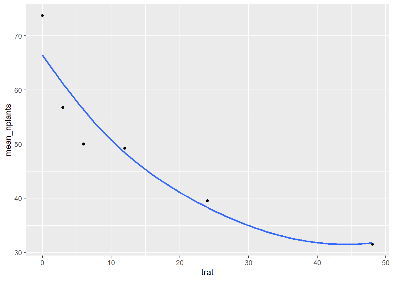
 estande2 |>
  ggplot(aes(trat, mean_nplants))+
  geom_point()+
# geom_line()+
   geom_smooth(method= "lm", se=FALSE, formula = y ~poly(x,2), color="black")+ #poly(x,2) já está transformando ao quadrado os valores
   theme_minimal()+
   annotate(geom="text", x = 25, y = 70, label = "y= 66.3 - 1777 + 0.0222x²
            R-squared = 0.88")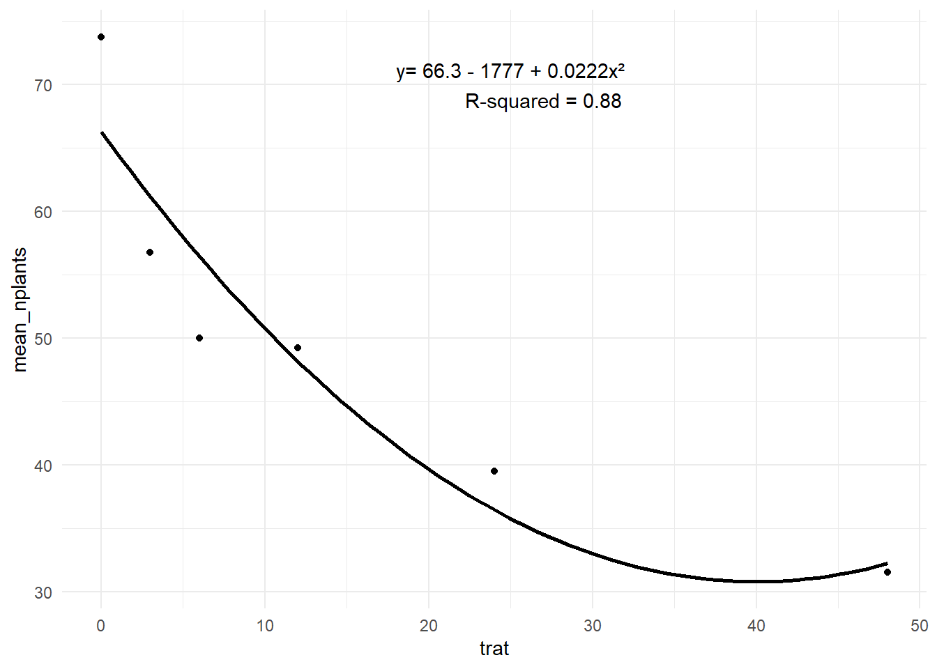
estande2 <- estande2 |>
  mutate(trat2 = trat^2)

m1 <- lm(mean_nplants ~ trat, data = estande2)
summary(m1)
Call:
lm(formula = mean_nplants ~ trat, data = estande2)

Residuals:
     1      2      3      4      5      6
12.764 -2.134 -6.782 -3.327 -4.669  4.147

Coefficients:
            Estimate Std. Error t value Pr(>|t|)
(Intercept)  60.9857     4.5505  13.402 0.000179 ***
trat         -0.7007     0.2012  -3.483 0.025294 *
---
Signif. codes:  0 '***' 0.001 '**' 0.01 '*' 0.05 '.' 0.1 ' ' 1

Residual standard error: 8.117 on 4 degrees of freedom
Multiple R-squared:  0.752, Adjusted R-squared:   0.69
F-statistic: 12.13 on 1 and 4 DF, p-value: 0.02529hist(m1$residuals)# r-squared: 0.69% da variaçao é explicado pela quantidade de inóculo assumindo o modelo linear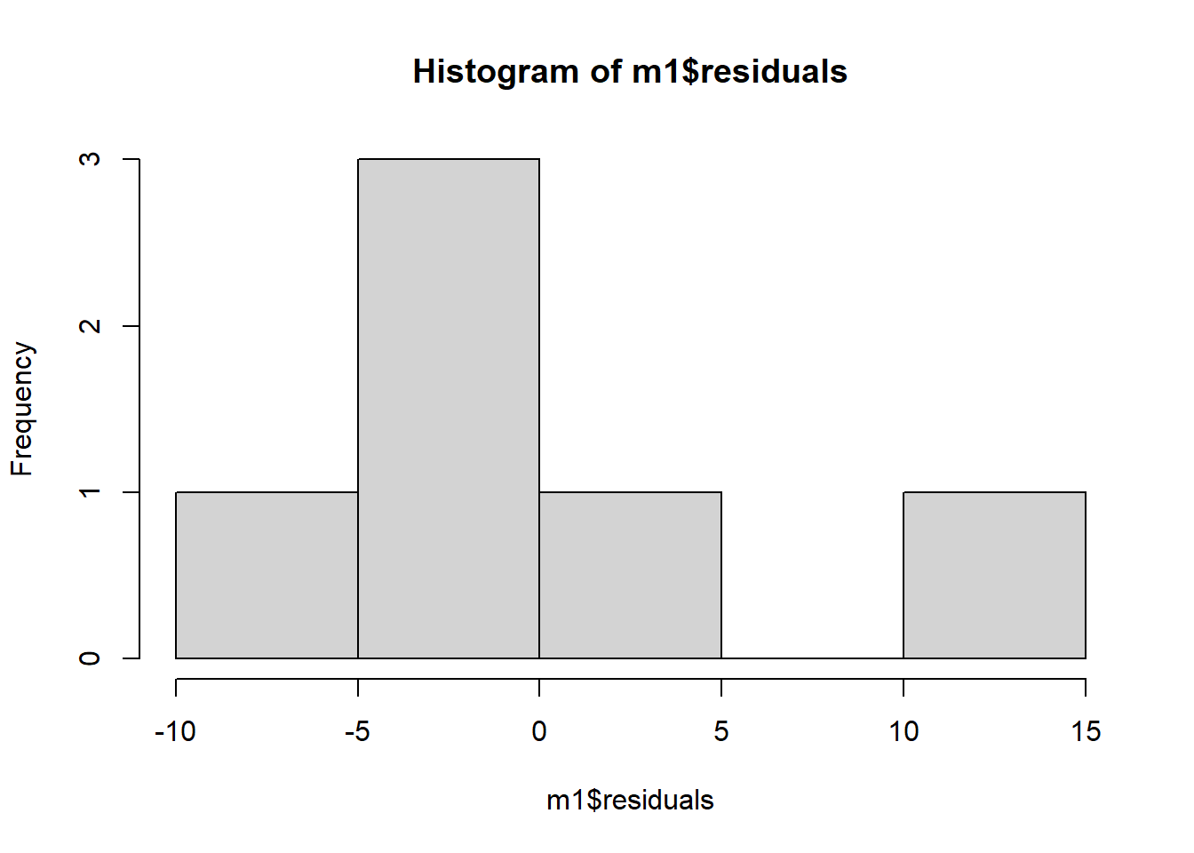
m2 <- lm(mean_nplants ~ trat + trat2, data = estande2) #criando modelo quadrático
summary(m2)  # Equação ficaria
Call:
lm(formula = mean_nplants ~ trat + trat2, data = estande2)

Residuals:
      1       2       3       4       5       6
 7.4484 -4.4200 -6.4386  1.0739  3.0474 -0.7111

Coefficients:
            Estimate Std. Error t value Pr(>|t|)
(Intercept) 66.30156    4.70800  14.083 0.000776 ***
trat        -1.77720    0.62263  -2.854 0.064878 .
trat2        0.02223    0.01242   1.790 0.171344
---
Signif. codes:  0 '***' 0.001 '**' 0.01 '*' 0.05 '.' 0.1 ' ' 1

Residual standard error: 6.517 on 3 degrees of freedom
Multiple R-squared:  0.8801,    Adjusted R-squared:  0.8001
F-statistic: 11.01 on 2 and 3 DF, p-value: 0.04152hist(m2$residuals)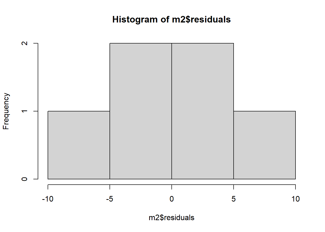
AIC(m1,m2) #o que der menor é melhor df AIC
m1 3 45.72200
m2 4 43.36151Agora com duas variáveis respostas do tipo numerica continua (quantitativa)
Realação entre duas variaveis respostas.
1 coisa: testar se tem associação entre as variaveis respostas.
R-square (R²): coficiente de determinação (quanto da variabilidade do y é explicada pela variação do x)
agora vamos fazer analise de correlação pearson (R): (é a raiz do R²) onde assumimos normalidade
mofo <- read_excel("dados-diversos.xlsx",
                   "mofo")

mofo |>
  ggplot(aes(inc, yld))+
  geom_point()+
  geom_smooth(method= "lm", se= FALSE)+
  facet_wrap(~ study)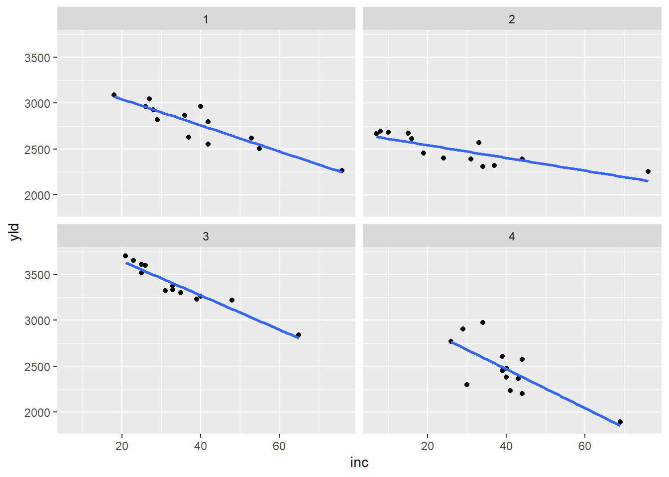
mofo1 <- mofo |>
  filter(study == 1)
mofo1
# A tibble: 13 × 5
study treat inc scl yld
<dbl> <dbl> <dbl> <dbl> <dbl>
1 1 1 76 2194 2265
2 1 2 53 1663 2618
3 1 3 42 1313 2554
4 1 4 37 1177 2632
5 1 5 29 753 2820
6 1 6 42 1343 2799
7 1 7 55 1519 2503
8 1 8 40 516 2967
9 1 9 26 643 2965
10 1 10 18 400 3088
11 1 11 27 643 3044
12 1 12 28 921 2925
13 1 13 36 1196 2867cor.test(mofo1$inc, mofo1$yld) #correlação negagtiva e significativa (vc olha no p-value se é sgnificativa)
    Pearson's product-moment correlation

data:  mofo1$inc and mofo1$yld
t = -6.8451, df = 11, p-value = 2.782e-05
alternative hypothesis: true correlation is not equal to 0
95 percent confidence interval:
 -0.9699609 -0.6921361
sample estimates:
       cor
-0.8999278
pcor <- cor(mofo |> select(3:5)) #correlação de todos
library(corrplot)
corrplot(pcor, method = 'number', type = "lower")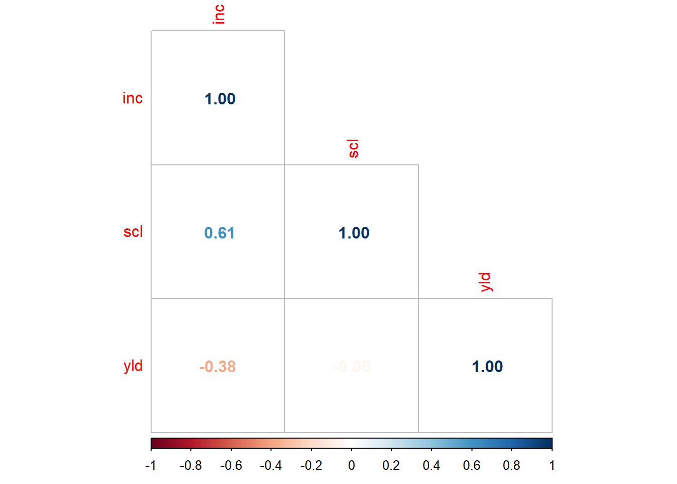
mofo1 # A tibble: 13 × 5
study treat inc scl yld
<dbl> <dbl> <dbl> <dbl> <dbl>
1 1 1 76 2194 2265
2 1 2 53 1663 2618
3 1 3 42 1313 2554
4 1 4 37 1177 2632
5 1 5 29 753 2820
6 1 6 42 1343 2799
7 1 7 55 1519 2503
8 1 8 40 516 2967
9 1 9 26 643 2965
10 1 10 18 400 3088
11 1 11 27 643 3044
12 1 12 28 921 2925
13 1 13 36 1196 2867shapiro.test(mofo$yld) # são normais pode usar pearson, se não fosse usava spearman
    Shapiro-Wilk normality test

data:  mofo$yld
W = 0.95769, p-value = 0.06216
mofo2 <- mofo |>
filter(study == 2)
mofo2# A tibble: 13 × 5
study treat inc scl yld
<dbl> <dbl> <dbl> <dbl> <dbl>
1 2 1 76 1331 2257
2 2 2 44 756 2393
3 2 3 24 338 2401
4 2 4 33 581 2568
5 2 5 37 588 2320
6 2 6 34 231 2308
7 2 7 31 925 2389
8 2 8 16 119 2614
9 2 9 10 394 2681
10 2 10 8 206 2694
11 2 11 15 275 2674
12 2 12 7 131 2666
13 2 13 19 588 2454cor.test(mofo2$inc, mofo2$yld)
    Pearson's product-moment correlation

data:  mofo2$inc and mofo2$yld
t = -4.6638, df = 11, p-value = 0.0006894
alternative hypothesis: true correlation is not equal to 0
95 percent confidence interval:
 -0.9426562 -0.4790750
sample estimates:
       cor
-0.8149448
pcor <- cor(mofo2 |> select(3:5), method = "spearman") #correlação de todos, usa spearman quando os dados não são normais.
library(corrplot)
corrplot(pcor, method = 'number', type = "lower")# associação de - 0.81 é uma associação forte e neste caso negativa e significativa segundo o p-value #spearman pra quando não tem normalidade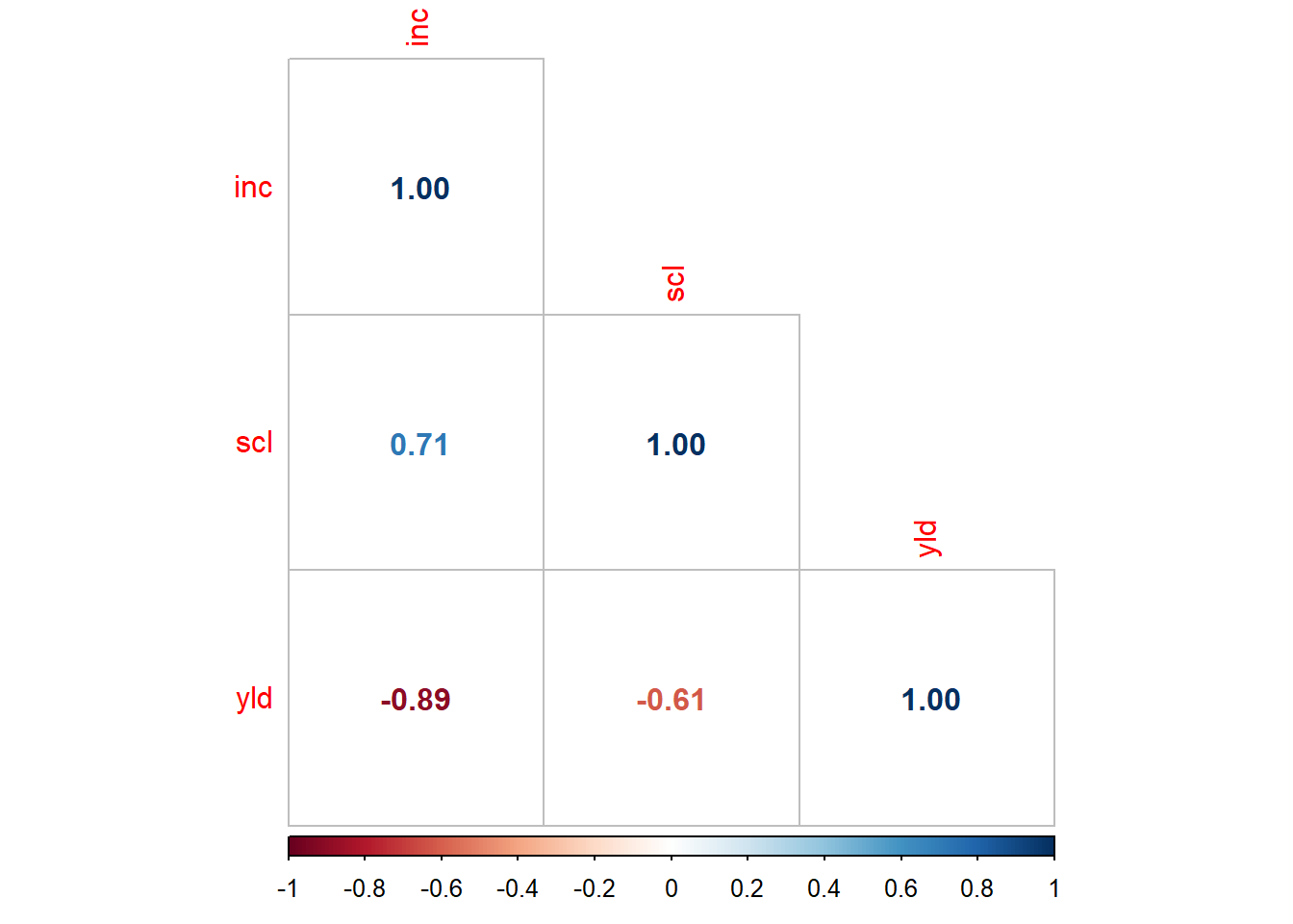
mofo4<- mofo |>
  filter(study == 4)
mofo4
# A tibble: 13 × 5
study treat inc scl yld
<dbl> <dbl> <dbl> <dbl> <dbl>
1 4 1 69 6216 1893
2 4 2 39 2888 2451
3 4 3 41 2272 2232
4 4 4 39 2868 2609
5 4 5 40 2412 2383
6 4 6 40 2372 2480
7 4 7 44 3424 2577
8 4 8 43 1744 2367
9 4 9 26 1456 2769
10 4 10 29 1732 2907
11 4 11 30 1080 2298
12 4 12 34 1592 2976
13 4 13 44 3268 2200cor.test(mofo4$inc, mofo4$yld)
    Pearson's product-moment correlation

data:  mofo4$inc and mofo4$yld
t = -3.7242, df = 11, p-value = 0.003357
alternative hypothesis: true correlation is not equal to 0
95 percent confidence interval:
 -0.9194503 -0.3327077
sample estimates:
       cor
-0.7467931