library(readxl)
library(tidyverse)
library(ggplot2)

fung <- read_excel("fung_myc.xlsx")

library(DT)
datatable(fung)Data analysis
The analysis of data from the in vitro experiment was conducted as follows:
#exploratory analysis

fung2 <- fung |>
  group_by(fungicide, dose, time) |>
  summarise(growth_mean = mean(growth))


pfung2 <- fung2 |>
   ggplot(aes(dose, growth_mean, group = time,
              color = factor(time)))+
  geom_point()+
  geom_line()+
  facet_wrap(~fungicide) +
      scale_y_continuous(n.breaks = 5, limits = c(0,5)) +
      labs(x = "Dose (μg a.i. mL)", y = "Mycelial growth (cm)", title= "Effect of fungicides on mycelial growth", color = "Experiment" ) +
      theme_minimal()+
    theme(plot.title = element_text(hjust = 0.5))

pfung2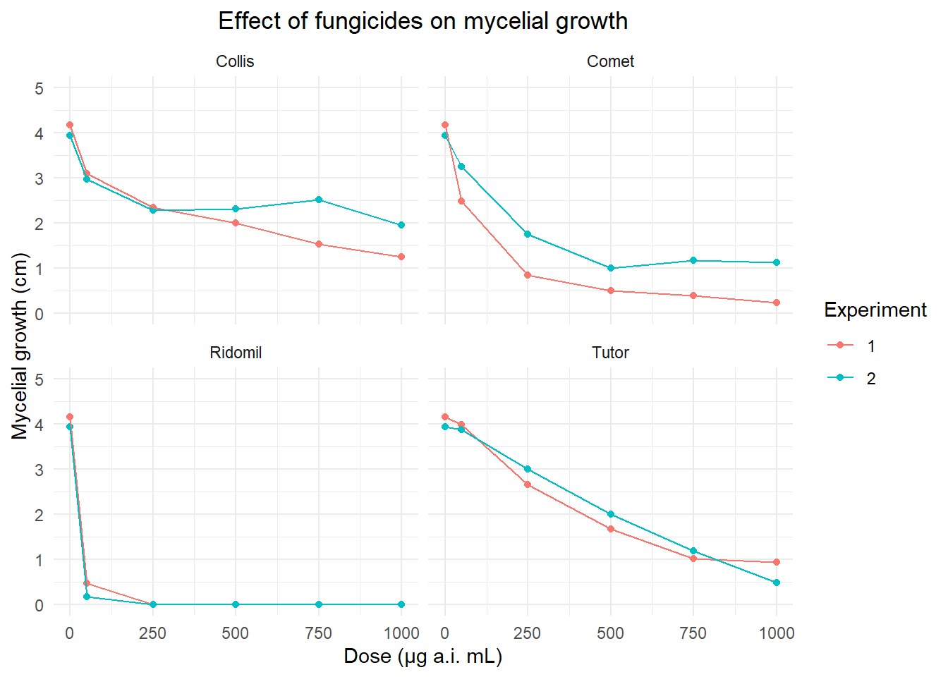
library(ggplot2)
library(dplyr)
library(patchwork)

fung2 <- fung |>
  group_by(fungicide, dose, time) |>
  summarise(growth_mean = mean(growth))

# Criaremos um gráfico separado para cada fungicida usando purrr::map e salvaremos os gráficos em uma lista

library(purrr)

# Vetor com os rótulos para cada fungicida
anotations <- c("EC50 = 67.26", "EC50 = 90.47", "EC50= 22 ", "EC50= 427.91")

plot_list <- fung2 %>%
  # Converter a coluna "fungicide" para fator e recodificar os nomes
  mutate(fungicide = factor(fungicide,
                            levels = c("Ridomil", "Comet", "Tutor", "Collis"),
                            labels = c("metalaxyl+mancozeb", "pyraclostrobin", "copper hydroxide", "boscalide+cresoxim-methyl"))) %>%
  group_by(fungicide) %>%
  group_split() %>%
  map2(anotations, ~{
    p <- ggplot(data = .x, aes(dose, growth_mean, group = time, color = factor(time))) +
      geom_point() +
      geom_line() +
      scale_y_continuous(n.breaks = 5, limits = c(0, 5)) +
      labs(x = "Dose (μg a.i. mL)", y = "Mycelial growth (cm)",
           title = paste(unique(.x$fungicide)),
           color = "Experiment") +
      theme_minimal() +
      theme(
        plot.title = element_text(size = 10, hjust = 0.5),
        axis.text.x = element_text(size = 7),
        axis.text.y = element_text(size = 7),
        axis.title.x = element_text(size = 7),
        axis.title.y = element_text(size = 7),
        legend.title = element_text(size = 7),
        legend.text = element_text(size = 7),
        plot.subtitle = element_text(size = 7),
        plot.caption = element_text(size = 5)
      )

    p <- p + annotate("text", x = Inf, y = Inf, hjust = 1, vjust = 1,
                      label = .y, size = 2.5, color = "black")

    return(p)
  })

# Use o patchwork para unir os gráficos
final_plot <- wrap_plots(plotlist = plot_list)

# Imprimir o gráfico final
print(final_plot)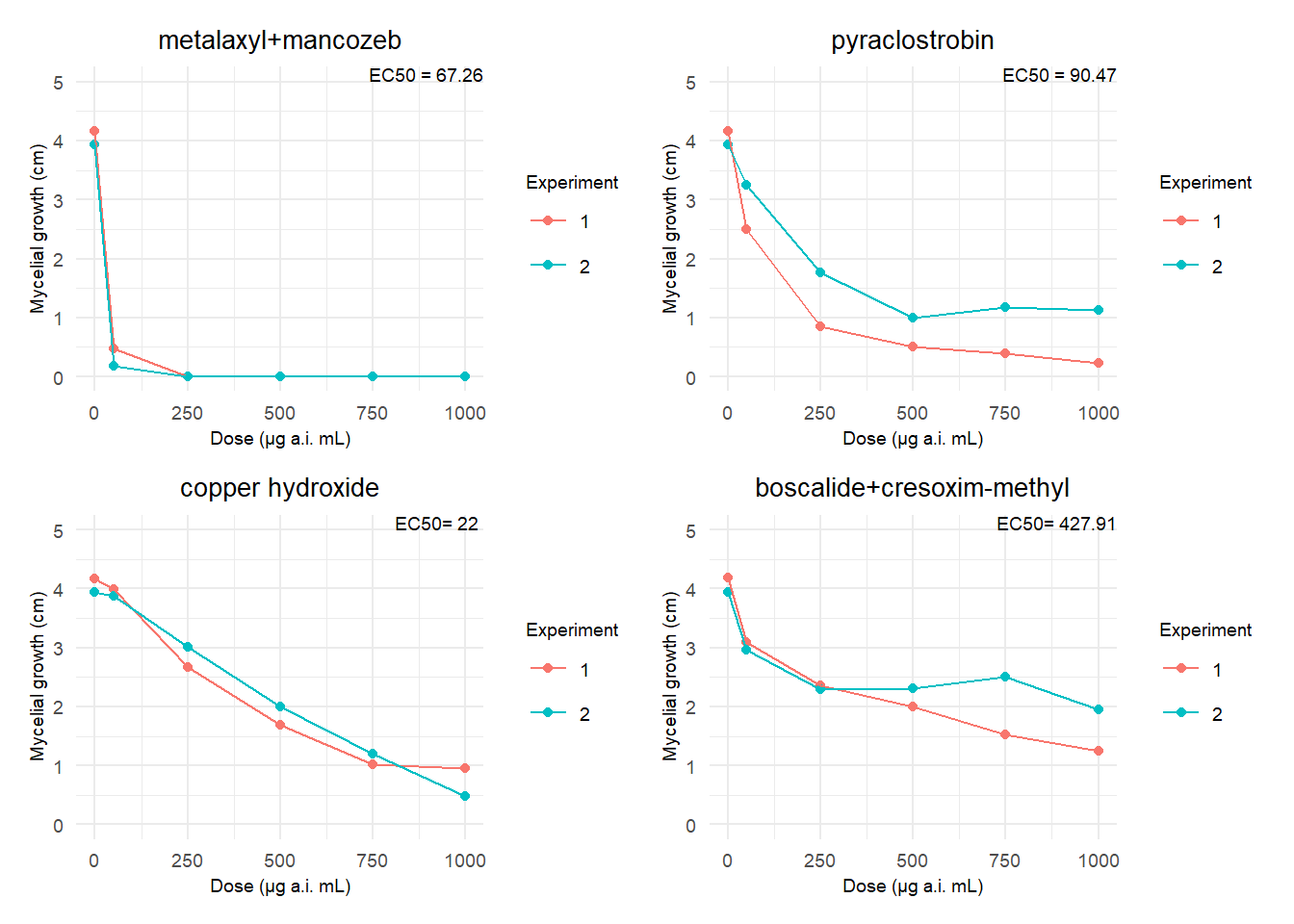
ggsave("finalplot_vitro.png",
bg = "white", width = 6, height= 4)library(ggplot2)
library(dplyr)
library(patchwork)
# Seu código para calcular o fung2 permanece o mesmo
fung2 <- fung |>
group_by(fungicide, dose, time) |>
summarise(growth_mean = mean(growth))
# Criaremos um gráfico separado para cada fungicida usando purrr::map e salvaremos os gráficos em uma lista
library(purrr)
# Vetor com os rótulos para cada fungicida
anotations <- c("EC50 = 67.26", "EC50 = 90.47", "EC50= 22 ", "EC50= 427.91")
plot_list <- fung2 %>%
group_by(fungicide) %>%
group_split() %>% # Corrigindo o uso do group_split
map2(anotations, ~{
# Criar o gráfico individual para cada fungicida
p <- ggplot(data = .x, aes(dose, growth_mean, group = time, color = factor(time))) +
geom_point() +
geom_line() +
scale_y_continuous(n.breaks = 5, limits = c(0, 5)) +
labs(x = "Dose (μg a.i. mL)", y = "Mycelial growth (cm)",
title = paste(unique(.x$fungicide)),
color = "Experiment") +
theme_minimal() +
theme(
plot.title = element_text(size = 10, hjust = 0.5), # Tamanho do título do gráfico
axis.text.x = element_text(size = 7), # Tamanho do texto do eixo x
axis.text.y = element_text(size = 7), # Tamanho do texto do eixo y
axis.title.x = element_text(size = 7), # Tamanho do título do eixo x
axis.title.y = element_text(size = 7), # Tamanho do título do eixo y
legend.title = element_text(size = 7), # Tamanho do título da legenda
legend.text = element_text(size = 7), # Tamanho do texto da legenda
plot.subtitle = element_text(size = 7), # Tamanho do texto da anotação
# Diminuir o tamanho da fonte da anotação específica para cada gráfico
plot.caption = element_text(size = 5)
)
# Adicionando a anotação de texto no gráfico com o rótulo correspondente ao fungicida
p <- p + annotate("text", x = Inf, y = Inf, hjust = 1, vjust = 1,
label = .y, size = 2.5, color = "black")
# Retornar o gráfico atualizado
return(p)
})
# Use o patchwork para unir os gráficos
final_plot <- wrap_plots(plotlist = plot_list)
# Imprimir o gráfico final
print(final_plot)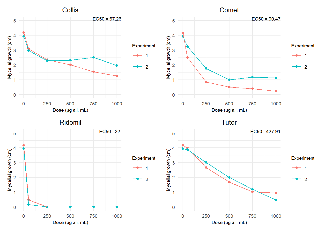
ggsave("plot_vitro.png",
          bg = "white", width = 6, height= 4)
Model fitting
library(dplyr)
library(drc)

#Ridomil
Ridomil <- fung2 |>
  filter(fungicide == "Ridomil")

drcrid <- drm(growth_mean ~ dose, data = Ridomil,
    fct = LL.3())  #Dose-Response Analysis
AIC(drcrid) #AIC (Akaike Information Criterion) é uma medida estatística que avalia a qualidade relativa de um modelo estatístico
[1] -19.175summary(drcrid)
Model fitted: Log-logistic (ED50 as parameter) with lower limit at 0 (3 parms)

Parameter estimates:

               Estimate Std. Error t-value   p-value
b:(Intercept)  2.961748   9.264597  0.3197    0.7565
d:(Intercept)  4.052506   0.063675 63.6436 2.945e-13 ***
e:(Intercept) 21.999862  56.542627  0.3891    0.7063
---
Signif. codes:  0 '***' 0.001 '**' 0.01 '*' 0.05 '.' 0.1 ' ' 1

Residual standard error:

0.0900501 (9 degrees of freedom)plot(drcrid)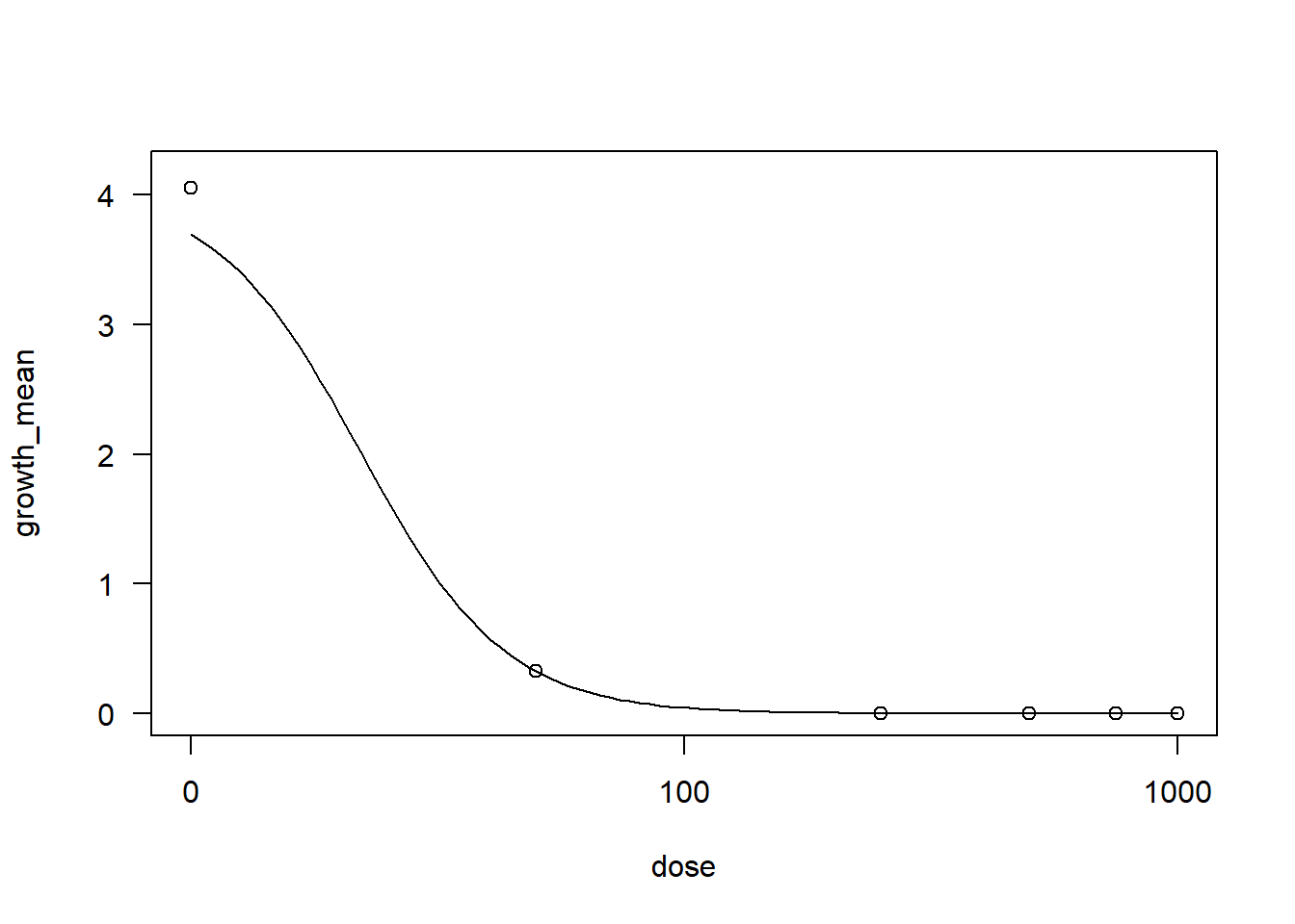
#LL.3() refere-se a uma função log-logística de três parâmetros, comumente usada para modelar respostas a doses crescentes#Collis
Collis <- fung2 |>
filter(fungicide == "Collis")
drccol3 <- drm(growth_mean ~ dose, data = Collis,
fct = LL.3())
AIC(drccol3)[1] 11.25187summary(drccol3)
Model fitted: Log-logistic (ED50 as parameter) with lower limit at 0 (3 parms)

Parameter estimates:

               Estimate Std. Error t-value  p-value
b:(Intercept)   0.45154    0.11974  3.7711 0.004409 **
d:(Intercept)   4.05505    0.22611 17.9340 2.37e-08 ***
e:(Intercept) 553.36080  195.38485  2.8322 0.019653 *
---
Signif. codes:  0 '***' 0.001 '**' 0.01 '*' 0.05 '.' 0.1 ' ' 1

Residual standard error:

0.319946 (9 degrees of freedom)plot(drccol3)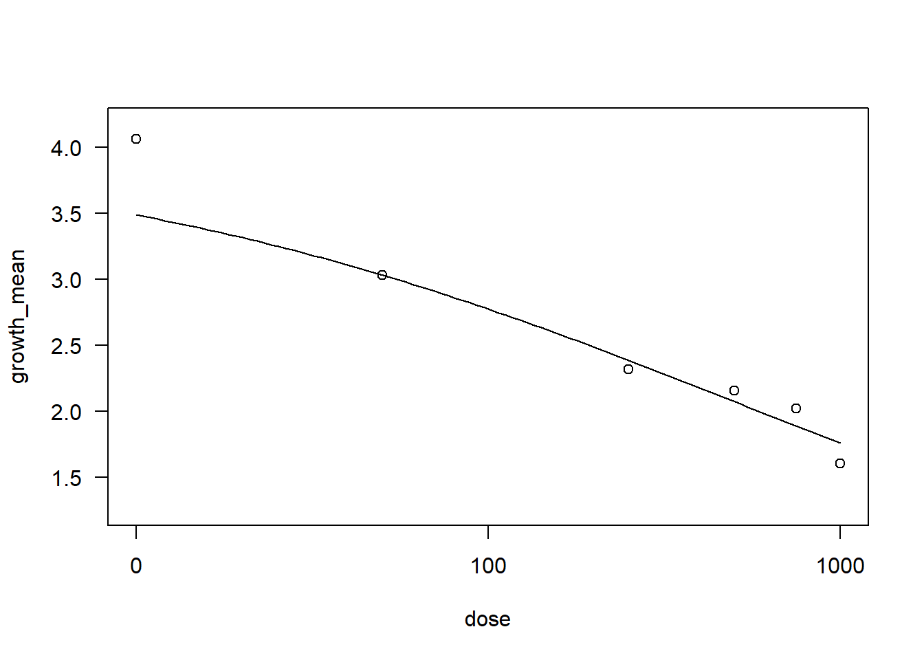
#apenas explorando sem a dose 0 pra ver se ajusta o modelo

Collis2 <- fung2 %>% filter(dose != "0") |>
  filter(fungicide == "Collis")

drccol2 <- drm(growth_mean ~ dose, data = Collis2,
    fct = LL.3())
AIC(drccol2)
[1] 12.18485summary(drccol2)
Model fitted: Log-logistic (ED50 as parameter) with lower limit at 0 (3 parms)

Parameter estimates:

                Estimate Std. Error t-value p-value
b:(Intercept)    0.54979    0.68631  0.8011  0.4494
d:(Intercept)    3.64932    2.05307  1.7775  0.1187
e:(Intercept)  844.60241 1645.42755  0.5133  0.6235

Residual standard error:

0.3565222 (7 degrees of freedom)plot(drccol2)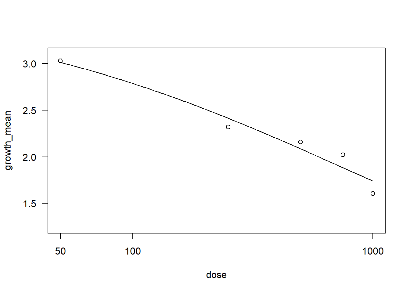
#Model modification

Collis <- fung2 |>
  filter(fungicide == "Collis")

drccol <- drm(growth_mean ~ dose, data = Collis,
    fct = EXD.3()) #EXP.3:O modelo assume uma relação exponencial entre a resposta e a dose, com três parâmetros estimados para capturar a forma da curva de resposta.
AIC(drccol)
[1] 15.16586summary(drccol)
Model fitted: Shifted exponential decay (3 parms)

Parameter estimates:

              Estimate Std. Error t-value   p-value
c:(Intercept)  1.96620    0.17502 11.2338 1.348e-06 ***
d:(Intercept)  3.98746    0.30126 13.2361 3.326e-07 ***
e:(Intercept) 97.04314   72.46426  1.3392    0.2133
---
Signif. codes:  0 '***' 0.001 '**' 0.01 '*' 0.05 '.' 0.1 ' ' 1

Residual standard error:

0.3766195 (9 degrees of freedom)plot(drccol)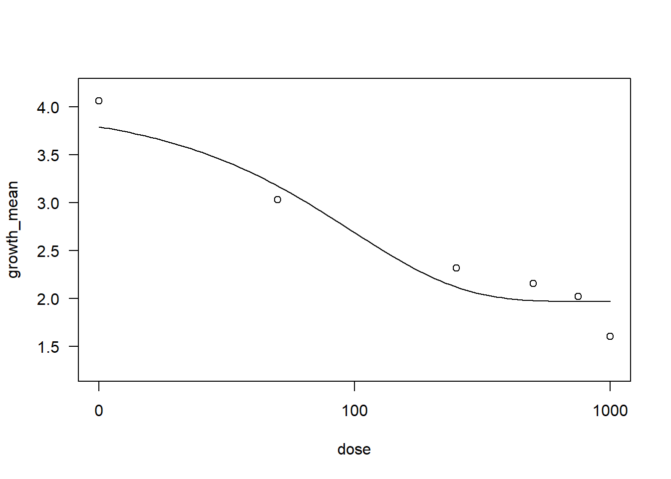
#Tutor
Tutor <- fung2 |>
  filter(fungicide == "Tutor")

drctut <- drm(growth_mean ~ dose, data = Tutor,
    fct = LL.3())
AIC(drctut)
[1] -2.736017summary(drctut)
Model fitted: Log-logistic (ED50 as parameter) with lower limit at 0 (3 parms)

Parameter estimates:

                Estimate Std. Error t-value   p-value
b:(Intercept)   1.703164   0.170555   9.986 3.620e-06 ***
d:(Intercept)   4.038278   0.099448  40.607 1.659e-11 ***
e:(Intercept) 427.910007  26.487305  16.155 5.913e-08 ***
---
Signif. codes:  0 '***' 0.001 '**' 0.01 '*' 0.05 '.' 0.1 ' ' 1

Residual standard error:

0.1786313 (9 degrees of freedom)plot(drctut)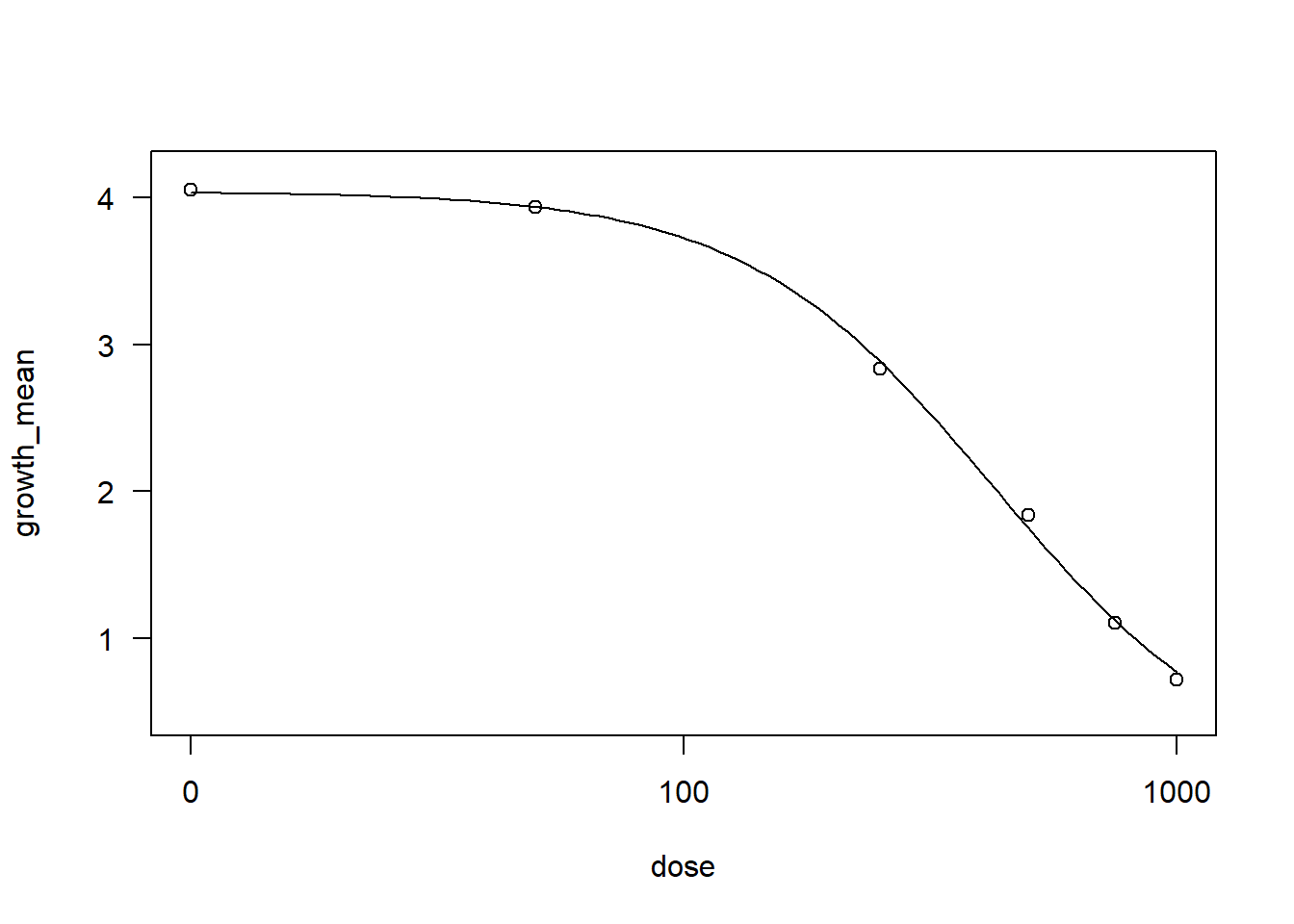
#Comet
Comet <- fung2 |>
  filter(fungicide == "Comet")

drccom2 <- drm(growth_mean ~ dose, data = Comet,
    fct = LL.3())
AIC(drccom2)
[1] 18.56011summary(drccom2)
Model fitted: Log-logistic (ED50 as parameter) with lower limit at 0 (3 parms)

Parameter estimates:

               Estimate Std. Error t-value   p-value
b:(Intercept)   0.89510    0.18828  4.7541  0.001038 **
d:(Intercept)   4.07136    0.30265 13.4525 2.893e-07 ***
e:(Intercept) 121.70989   37.58603  3.2382  0.010188 *
---
Signif. codes:  0 '***' 0.001 '**' 0.01 '*' 0.05 '.' 0.1 ' ' 1

Residual standard error:

0.4338342 (9 degrees of freedom)plot(drccom2)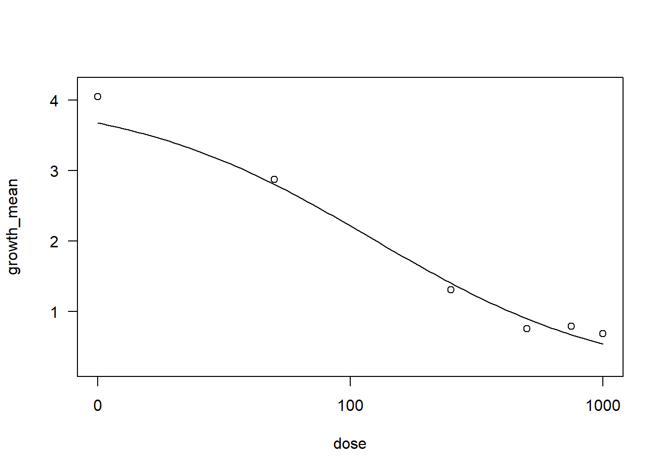
drccom <- drm(growth_mean ~ dose, data = Comet,
    fct = EXD.3())
AIC(drccom)
[1] 17.92899summary(drccom)
Model fitted: Shifted exponential decay (3 parms)

Parameter estimates:

               Estimate Std. Error t-value   p-value
c:(Intercept)   0.72856    0.19049  3.8247  0.004061 **
d:(Intercept)   4.00455    0.28239 14.1807 1.836e-07 ***
e:(Intercept) 130.52175   43.37518  3.0091  0.014737 *
---
Signif. codes:  0 '***' 0.001 '**' 0.01 '*' 0.05 '.' 0.1 ' ' 1

Residual standard error:

0.4225745 (9 degrees of freedom)plot(drccom)
EC50
erid <- ED(drcrid, 50, interval = "delta") #ridomil
Estimated effective doses

       Estimate Std. Error    Lower    Upper
e:1:50   22.000     56.543 -105.908  149.908
ecol <- ED(drccol, 50, interval = "delta") #collis
Estimated effective doses

       Estimate Std. Error   Lower   Upper
e:1:50   67.265     50.228 -46.359 180.890
etut <- ED(drctut, 50, interval = "delta") #tutor
Estimated effective doses

       Estimate Std. Error   Lower   Upper
e:1:50  427.910     26.487 367.992 487.828
ecom <- ED(drccom, 50, interval = "delta") #comet
Estimated effective doses
Estimate Std. Error Lower Upper
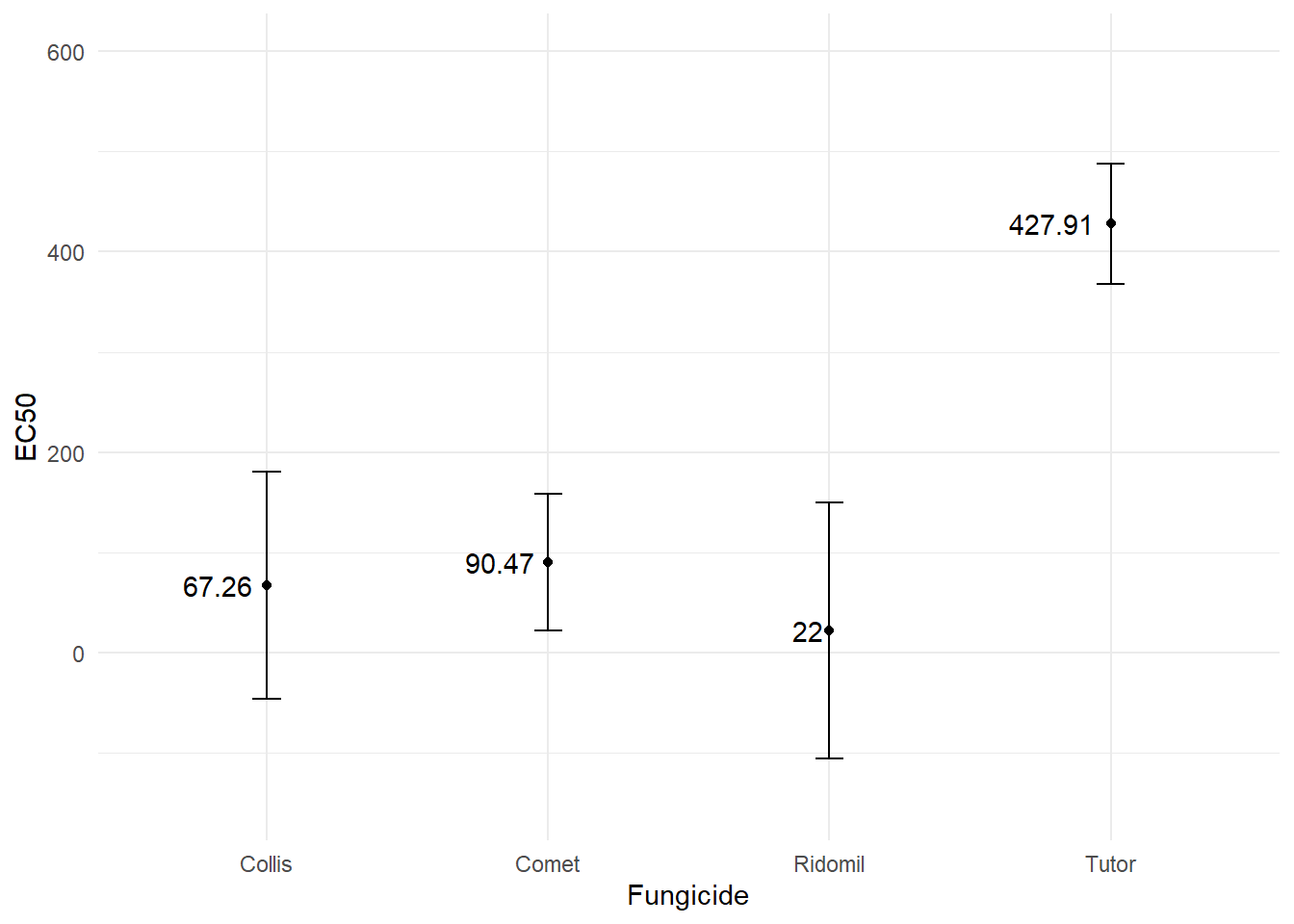
e:1:50 90.471 30.065 22.458 158.483dadosec <- data.frame( Trat = c("Ridomil", "Collis", "Tutor", "Comet"),
Estimate = c(22.00, 67.265, 427.910, 90.471),
Lower = c(-105.908, -46.359, 367.992, 22.458),
Upper = c(149.908, 180.890, 487.828, 158.483))
datatable(dadosec)library(ggplot2)
plotEC <- dadosec |>
ggplot(aes(Trat, Estimate)) +
geom_point() +
ylim(-150,600)+
geom_errorbar(aes(ymin = Lower, ymax = Upper), width = 0.1) +
geom_text(aes(label = round(Estimate, 2)), hjust = 1.2) +
labs(x = "Fungicide", y = "EC50") +
theme_minimal()
plotEC