Data analysis

The analysis of data from the in vivo experiment was conducted as follows:

library(readxl)
library(tidyverse)
library(car)
library(performance)
library(DT)

vivo <- read_excel("fung_invivo.xlsx")

library(DT)
datatable(vivo)

# Removing Control
vivo2 <- vivo %>% filter(treatment != "Control")


m <- lm(lesion ~ cultivar*treatment*time, data = vivo2)
Anova(m) #First, we checked if the interaction of cultivar*treatment*time was significant: It was not.

Anova Table (Type II tests)

Response: lesion
                        Sum Sq Df F value    Pr(>F)    
cultivar                 172.4  1  2.0622    0.1575    
treatment                 84.5  2  0.5055    0.6064    
time                    3733.5  1 44.6651 2.251e-08 ***
cultivar:treatment        59.4  2  0.3551    0.7029    
cultivar:time             27.6  1  0.3303    0.5682    
treatment:time             2.5  2  0.0152    0.9849    
cultivar:treatment:time    6.5  2  0.0390    0.9617    
Residuals               4012.3 48                      
---
Signif. codes:  0 '***' 0.001 '**' 0.01 '*' 0.05 '.' 0.1 ' ' 1

m1 <- lm(lesion ~ cultivar*treatment, data = vivo2)
Anova(m1)

Anova Table (Type II tests)

Response: lesion
                   Sum Sq Df F value Pr(>F)
cultivar            172.4  1  1.1961 0.2790
treatment            84.5  2  0.2932 0.7471
cultivar:treatment   59.4  2  0.2060 0.8145
Residuals          7782.5 54               

check_normality(m1)# The data approximately follow a normal distribution. Let's consider a significance level of p=0.05.

Warning: Non-normality of residuals detected (p < .001).

check_heteroscedasticity(m1)

OK: Error variance appears to be homoscedastic (p = 0.129).

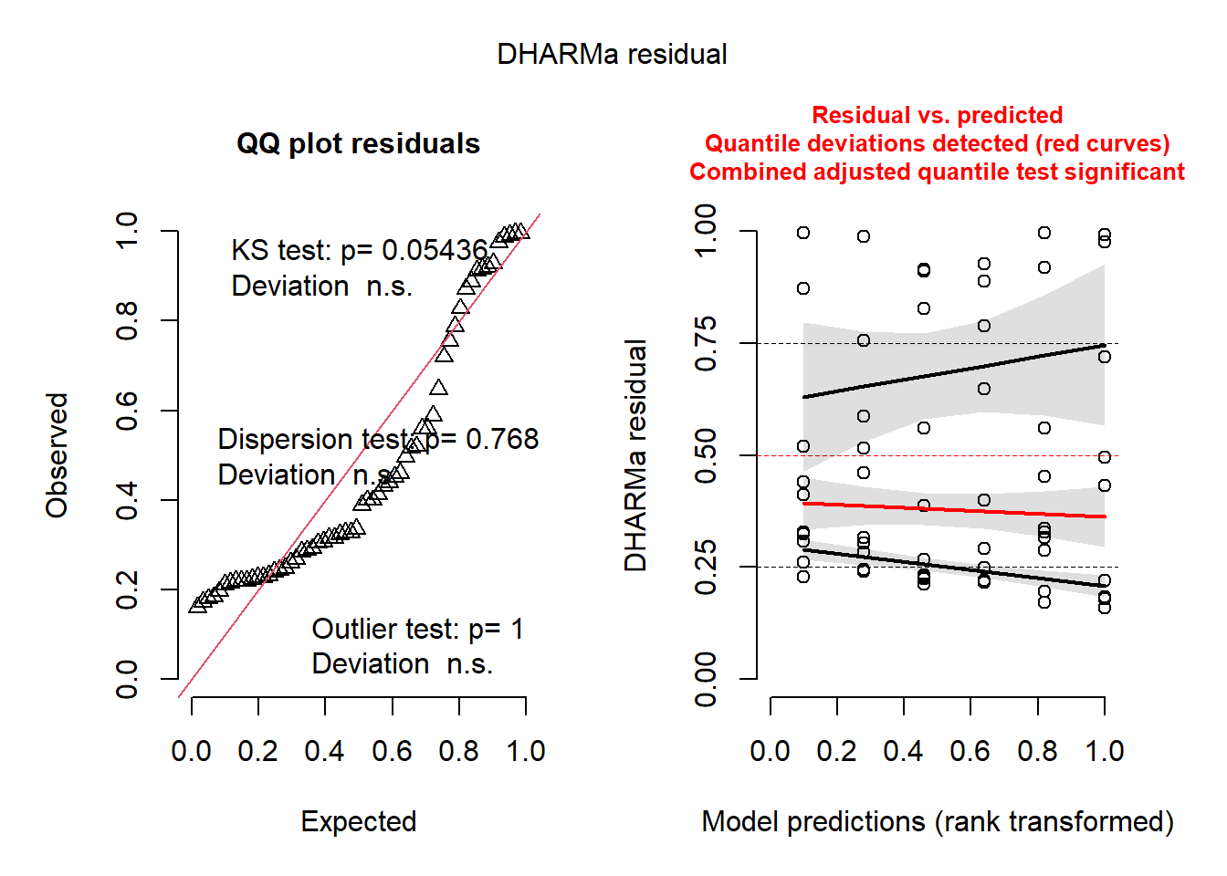
library(DHARMa)
plot(simulateResiduals(m1))

Transformando os dados com log

m2 <- lm(log(lesion) ~ cultivar*treatment, data = vivo2)

# Analysis of variance (ANOVA) for model m1
library(car)
Anova(m2)

Anova Table (Type II tests)

Response: log(lesion)
                   Sum Sq Df F value Pr(>F)
cultivar            1.497  1  1.6849 0.1998
treatment           0.835  2  0.4701 0.6275
cultivar:treatment  0.641  2  0.3609 0.6987
Residuals          47.984 54               

check_normality(m2)# The data approximately follow a normal distribution. Let's consider a significance level of p=0.05.

Warning: Non-normality of residuals detected (p = 0.011).

check_heteroscedasticity(m2)

OK: Error variance appears to be homoscedastic (p = 0.559).

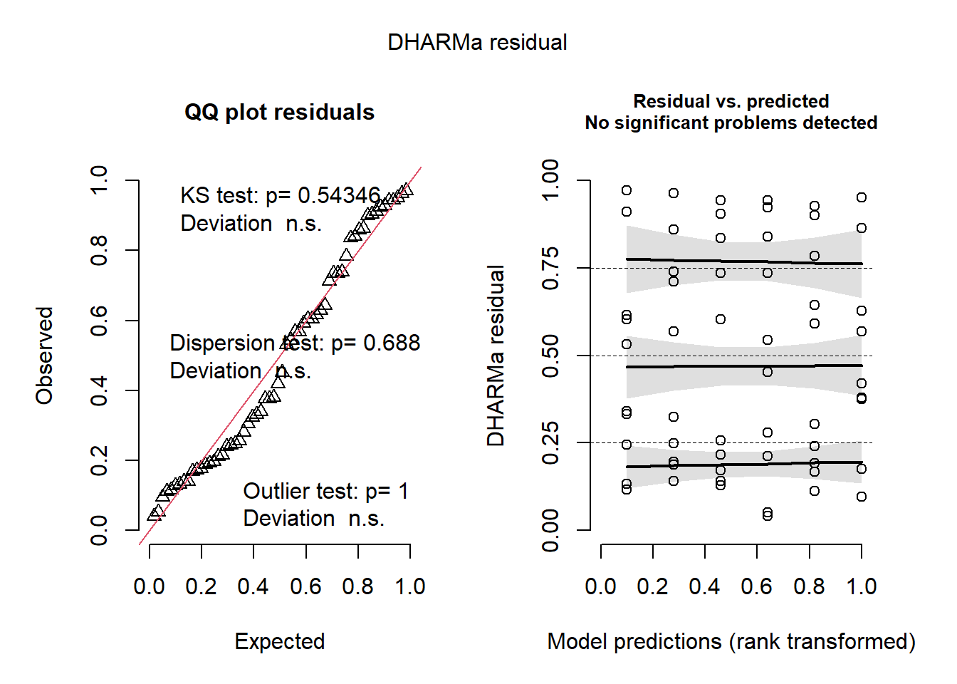
library(DHARMa)
plot(simulateResiduals(m2))

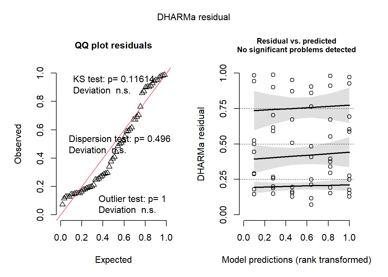
#poderia usar tbm o glm, ao inves de lm com transformação, ajuste do modelo linear não generalizado
mglm <- glm(lesion ~cultivar*treatment, data = vivo2,
            family = Gamma) #tamanho da lesão é um valor sempre maior que 0 e tem uma distribuição gama
plot(simulateResiduals(mglm))

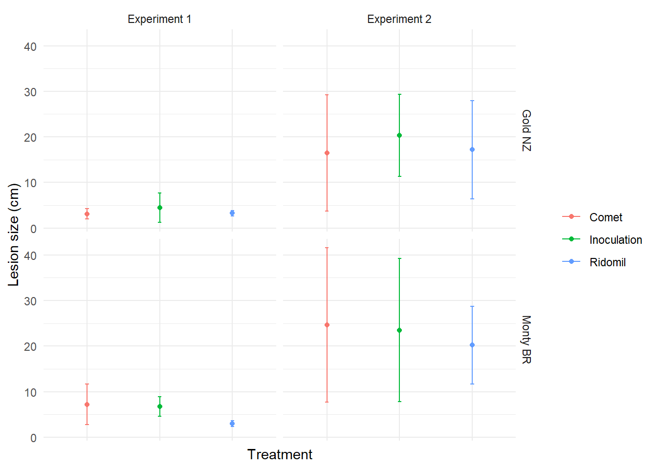
Analysis of variance (ANOVA) showed that cultivar (p = 0.19), fungicide treatment (p= 0.67), and the interaction between cultivar and treatment had no significant effect on lesion size (p = 0.69). Most of the variability was attributed to residues (Sum Sq = 47.984).

library(ggplot2)
library(dplyr)
library(forcats)

fungvivo <- vivo2  |>
  group_by(treatment, cultivar, time) |> 
  summarise(lesion_mean = mean(lesion), 
            lesion_sd = sd(lesion)) 

datatable(fungvivo)

# Converter a coluna "time" em fator
fungvivo$time <- factor(fungvivo$time)

# Renomear os níveis da variável "time" usando fct_recode
fungvivo$time <- fct_recode(fungvivo$time,
                            "Experiment 1" = "1",
                            "Experiment 2" = "2")

plotvivo <- fungvivo |> 
  ggplot(aes(treatment, lesion_mean, color = treatment)) +
  facet_wrap(~cultivar) +
  geom_point() +
  geom_errorbar(aes(ymin = lesion_mean - lesion_sd, ymax = lesion_mean + lesion_sd, width = 0.05)) +
  facet_grid(cultivar ~ time) +
  theme_minimal() +
  theme(plot.title = element_text(hjust = 0.5)) +  
  labs(x = "Treatment", y = "Lesion size (cm)") +
  guides(color = guide_legend(title = NULL))  # Removendo o título da legenda do eixo x

# Removendo os rótulos do eixo x (nomes dos tratamentos)
plotvivo <- plotvivo + scale_x_discrete(labels = NULL)

print(plotvivo)

ggsave("plot_vivo.png", bg = "white", width = 6, height = 4)

Figures

Lesion